2020/04/24 - [Opencv] - 간단한 손글씨 인식하기 -1
2020/04/30 - [Opencv] - 간단한 손글씨 인식하기 -2
2020/04/30 - [Opencv] - 간단한 손글씨 인식하기 -3
2020/05/04 - [Computer Vision/Classification] - MNIST 데이터를 이용해서 손글씨 인식하기
이 글은 앞의 포스팅을 하나로 묶어놓은 게시글임.
머신러닝을 통해 손글씨를 인식하기 위해 Opencv의 함수들과 scikit-learn의 ML기법들을 이용해서 전처리 부터 손글씨 인식 단계까지 진행해보고자 한다. 아래와 같이 직접 적은 글씨를 MNIST데이터를 통해 훈련시킨뒤에 이미지를 전처리해서 TEST하여 정확도를 확인하는 단계까지 진행하였다.
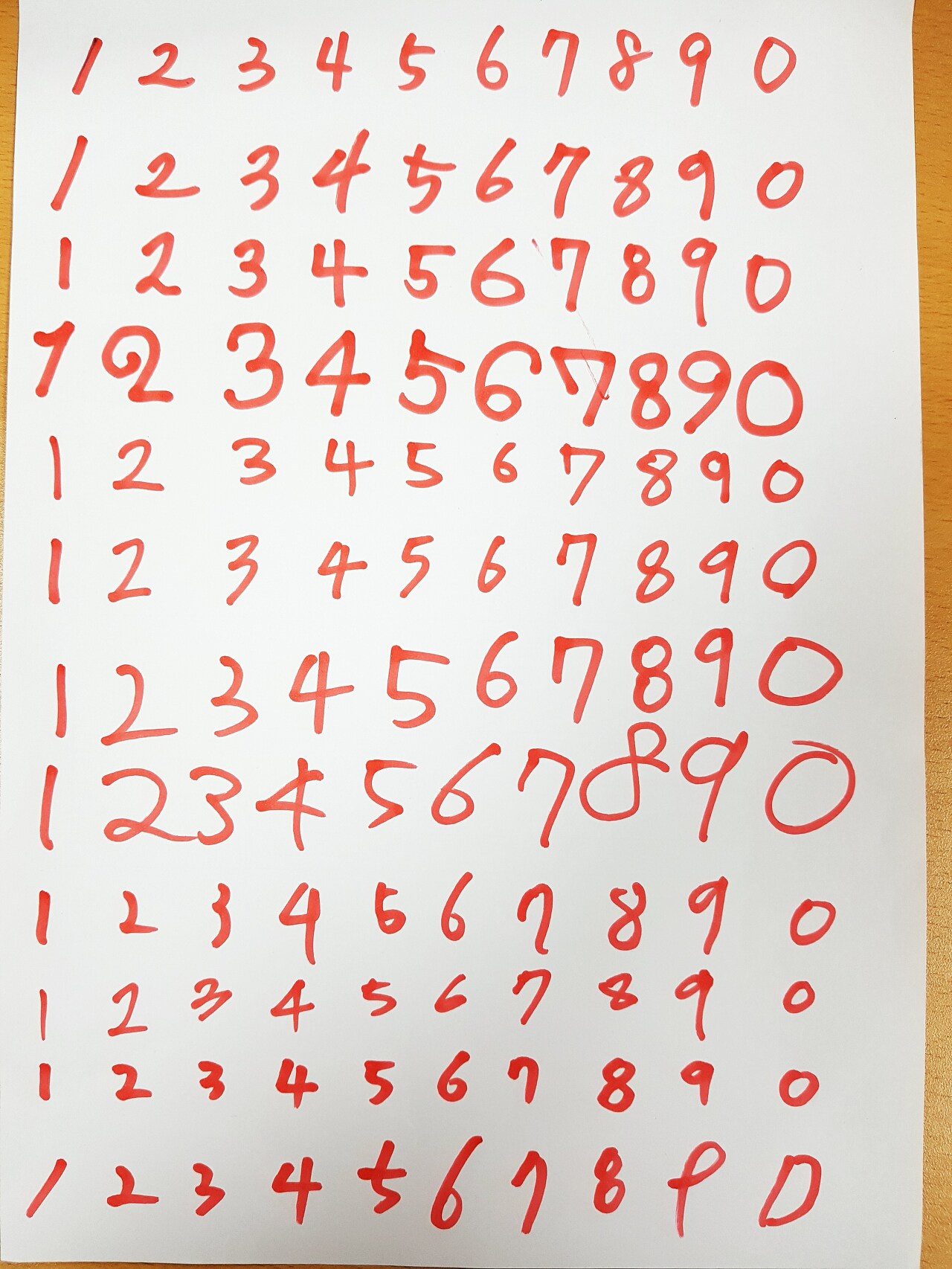
실제 데이터
먼저 손글씨를 훈련시키기 위해 txt파일로 이루어진 MNIST데이터를 받아왔다.
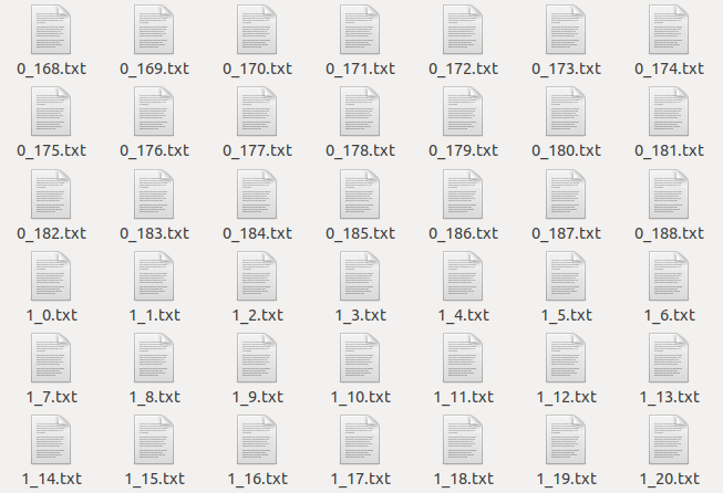
txt파일로 된 MNIST 데이터
이렇게 txt파일이 있고, 파일명은 label과 번호가 적혀있다. 이 txt파일의 내용을 보면,

데이터 3의 내용
이런식으로 0과 1로 이루어져 있는 txt파일이 존재한다. 우리가 이 훈련 데이터를 훈련시키기 위해서는 이걸 그대로 배열 형태로 변환해서 사용해도 되지만 실제 데이터로 test를 할 예정 이기도 하고, 이미지로 변환시켜주는 전처리를 연습도 할겸, 이미지로 먼저 변환을 해주었다.
양이 많지 않기 때문에 전처리하는 과정이 오래 걸리지 않지만, 만약 데이터의 양이 엄청나게 많아지면 전처리가 되어가는 진행도를 확인할 수 있으면 좋을 것 같아서 percentbar가 나올 수 있게 함수를 하나 만들어 주었다.
bar = '□□□□□□□□□□'	#퍼센트바의 초기 상태
sw = 1
def percent_bar(array,count):   #퍼센트를 표시해주는 함수
    global bar
    global sw
    length = len(array)
    percent = (count/length)*100	#배열의 길이와 현재 for문의 count의 퍼센트를 구함
    if count == 1 :
        print('preprocessing...txt -> png ')
    print('\r'+bar+'%3s'%str(int(percent))+'%',end='')	#퍼센트바와 퍼센트를 표시
    if sw == 1 :
        if int(percent) % 10 == 0 :
            bar = bar.replace('□','■',1)	#네모가 열개이므로 10퍼센트마다 한개씩 채워줌
            sw = 0
    elif sw == 0 :
        if int(percent) % 10 != 0 :
            sw = 1
다음은 txt로 되어있는 데이터 파일을 읽어서 png파일로 변경해주는 작업을 해주었다.
0과 1로 되어있기 때문에 0은 그대로 냅두고 1을 255로 변경하여 흰색으로 저장을 해주었다.
import os
import numpy as np

def preprocessing_txt(path):
    txtPaths = [os.path.join(path,f) for f in os.listdir(path)]
    count = 0
    #파일읽기
    for txtPath in txtPaths :
        count += 1
        filename = os.path.basename(txtPath)
        percent_bar(txtPaths,count)
        f = open(txtPath)
        img = []
        while True :
            tmp=[]
            text = f.readline()
            if not text :
                break
            for i in range(0,len(text)-1) :
                #라인을 일어올때 text가 1일경우 255로 변경
                if int(text[i]) == 1 :
                    tmp.append(np.uint8(255))
                else :
                    tmp.append(np.uint8(0))
            img.append(tmp)		#img배열에 쌓아줌
        img = np.array(img)
        cv2.imwrite('./kNN/trainingPNGs/'+filename.split('.')[0]+'.png',img) #저장
print('\n'+str(count)+'files are saved(preprocessing_txt2png)')preprocessing_txt('./kNN/trainingDigits')|
preprocessing...txt -> png ■■■■■■■■■■100% 1934files are saved(preprocessing_txt2png) |
실행하면 퍼센트바로 진행도를 확인할 수 있고, 몇장이 저장되었는지 print해두었다.
이 당시.. for문의 진행도를 표현하는 방법을 몰라 직접 코딩하였지만, tqdm을 쓰면 정말 편리하고 멋지게 확인이 가능하다..
그럼 이제 잘 저장 되었는지 확인해보자.

txt파일이 png파일로 전처리된 모습
확인해보면 txt파일이었던 데이터가 png파일로 변경되어 잘 저장된 것을 확인할 수 있다.
txt파일을 이미지 데이터로 변환해주었기 때문에 이번에는 실제 이미지인 digits.jpg를 전처리하여 각각의 이미지 파일과 labeling 하는 작업을 진행 해보도록 하겠다.

digits.jpg
먼저 opencv를 이용해서 grayscale로 해당 이미지를 불러온다.
import cv2
import numpy as np

filename = 'digits.jpg'

src = cv2.imread(filename,cv2.IMREAD_GRAYSCALE) #그레이 스케일로 변환
src = cv2.resize(src , (int(src.shape[1]/5),int(src.shape[0]/5)))
#이미지의 크기가 워낙 크기 때문에 5분의1로 줄여서 확인
cv2.imshow('gray',src)

k = cv2.waitKey(0)

cv2.destroyAllWindows()
그레이 스케일로 변환된 이미지
이제 그레이스케일 이미지를 이전의 MNIST이미지와 같은 형태로 만들기 위해 이진화 작업을 해주어야 한다. 이진화 작업을 진행할 때, 양옆이나 밑부분에 촬영된 나무바닥의 부분은 노이즈가 될 가능성이 크기 때문에 잘라주도록 하자.
src = src[0:src.shape[0]-10, 15:src.shape[1]-25] #양 옆의 노이즈를 제거
ret , binary = cv2.threshold(src,170,255,cv2.THRESH_BINARY_INV) #영상 이진화

cv2.imshow('binary',binary)

k = cv2.waitKey(0)

cv2.destroyAllWindows()
이진화 이미지
이미지의 손글씨를 하나하나 labeling하기 위해서는 외곽선 검출을 통해 box를 쳐서 분리해 내야 하는데 이진화 이미지를 보면 점이나 빛으로 인한 노이즈가 생긴것을 확인할 수 있다. 노이즈를 제거하기 위해 모폴로지 연산을 통해 제거해주자.
binary = cv2.morphologyEx(binary , cv2.MORPH_OPEN , cv2.getStructuringElement(cv2.MORPH_ELLIPSE, (2,2)), iterations = 2)

cv2.imshow('binary',binary)

k = cv2.waitKey(0)

cv2.destroyAllWindows()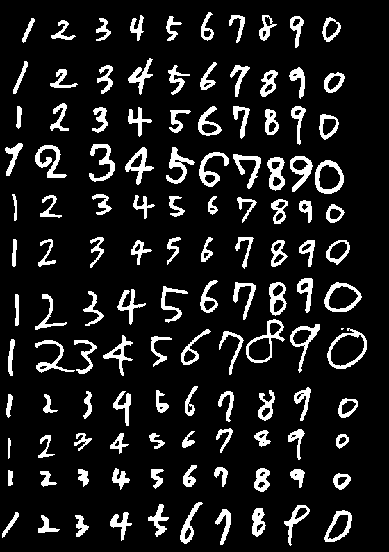
열기연산을 통해 노이즈 제거
노이즈를 제거 한 뒤에 opencv 의 findContours를 이용하여 외곽선 검출을 한 다음, boundingRect를 통해 사각형을 그려주면 손글씨의 숫자대로 나누어 줄 수 있다.
contours , hierarchy = cv2.findContours(binary , cv2.RETR_EXTERNAL , cv2.CHAIN_APPROX_SIMPLE)
#외곽선 검출
color = cv2.cvtColor(binary, cv2.COLOR_GRAY2BGR) #이진화 이미지를 color이미지로 복사(확인용)
cv2.drawContours(color , contours , -1 , (0,255,0),3) #초록색으로 외곽선을 그려준다.

#리스트연산을 위해 초기변수 선언
bR_arr = []
digit_arr = []
digit_arr2 = []
count = 0

#검출한 외곽선에 사각형을 그려서 배열에 추가
for i in range(len(contours)) :
    bin_tmp = binary.copy()
    x,y,w,h = cv2.boundingRect(contours[i])
    bR_arr.append([x,y,w,h])
사각형을 만들어서 손글씨를 나누어 주었지만 배열을 확인해보면 랜덤하게 박스가 생성되었다는 것을 알 수 있다.
print(bR_arr[:5])| [[229, 795, 3, 1], [55, 742, 33, 26], [109, 741, 20, 33], [4, 738, 25, 37], [159, 737, 32, 42]] |
이미지를 확인 해보면 x값이 작을 수록 숫자가 작다는 것을 알 수 있다. 그러므로 x값을 기준으로 오름차순 정렬을 해주면 숫자의 순서대로 정렬이 될 것 이다.
#x값을 기준으로 배열을 정렬
bR_arr = sorted(bR_arr, key=lambda num : num[0], reverse = False)

print(bR_arr[:5])| [[4, 738, 25, 37], [8, 206, 26, 48], [10, 568, 9, 34], [12, 677, 7, 24], [12, 631, 5, 30]] |
오름차순으로 정렬하여 숫자가 순서대로 배열에 담겨져 있다는 것으 알 수 있다. 이번엔 배열의 길이를 확인 해보자.
print(len(bR_arr))| 122 |
배열의 길이를 확인해봤더니 122개로 나오는 것을 알 수 있다. 12줄의 10개의 숫자를 적었으니 120개가 나와야하지만 2개의 작은 점으로 인해 노이즈데이터가 생성된 것을 확인 할 수 잇다. box를 그림으로 그려주면서 일정크기 이하의 box를 버려 노이즈를 제거하고 나머지는 이미지로 잘라내어 새로운 배열에 담아주었다.
#작은 노이즈데이터 버림,사각형그리기,12개씩 리스트로 다시 묶어서 저장
for x,y,w,h in bR_arr :
    tmp_y = bin_tmp[y-2:y+h+2,x-2:x+w+2].shape[0]
    tmp_x = bin_tmp[y-2:y+h+2,x-2:x+w+2].shape[1]
    if  tmp_x and tmp_y > 10 :
        count += 1
        cv2.rectangle(color,(x-2,y-2),(x+w+2,y+h+2),(0,0,255),1)
        digit_arr.append(bin_tmp[y-2:y+h+2,x-2:x+w+2])
        if count == 12 :
            digit_arr2.append(digit_arr)
            digit_arr = []
            count = 0

cv2.imshow('contours',color)

k = cv2.waitKey(0)
cv2.destroyAllWindows()
노이즈가 제거되고 숫자만 bounding box된 모습
이제 이것 들을 MNIST데이터와 같은 32x32 의 크기의 이미지로 저장해주도록 하자. 이때 파일이름에 label을 달아주기 위해 이중 for문을 이용하여 '{숫자}_{번호}.png'로 저장해 주었다.
#리스트에 저장된 이미지를 32x32의 크기로 리사이즈해서 순서대로 저장
for i in range(0,len(digit_arr2)) :
    for j in range(len(digit_arr2[i])) :
        count += 1
        if i == 0 :         #1일 경우 비율 유지를 위해 마스크를 만들어 그위에 얹어줌
            width = digit_arr2[i][j].shape[1]
            height = digit_arr2[i][j].shape[0]
            tmp = (height - width)/2
            mask = np.zeros((height,height))
            mask[0:height,int(tmp):int(tmp)+width] = digit_arr2[i][j]
            digit_arr2[i][j] = cv2.resize(mask,(32,32))
        else:
            digit_arr2[i][j] = cv2.resize(digit_arr2[i][j],(32,32))
        if i == 9 : i = -1
        cv2.imwrite('./kNN/testPNGs/'+str(i+1)+'_'+str(j)+'.png',digit_arr2[i][j])
하지만 저장될 때 1의 경우 bounding box 가 세로와 가로의비율 차이가 너무 커져서 이미지가 1인지 식별하기 힘들게 저장이 되기 때문에 1이라는 숫자의 비율유지를 위해 마스크이미지를 하나 생성하여 그 마스크 이미지에 비율이 유지되도록 이미지를 재생성하여 저장해주었다.

<- 마스크를 씌우기 전의 1의 이미지

<- 마스크를 씌운 뒤의 1의 이미지

손글씨 이미지가 MNIST데이터와 같은 형태로 저장된 모습
이제 전처리를 통해 training set과 test set을 모두 구비가 완료 되었으니 이번에는 scikit-learn을 이용하여 머신러닝을 통해 test셋을 MNIST데이터를 훈련시켜 맞춰보도록 하자.
가장 먼저, sckit-learn에 훈련 시킬 수 있게 train x와 y로 나누어 데이터 셋을 만드는 함수를 작성 하였다.
def createdataset(directory):       #sklearn사용을 위해 데이터세트를 생성
    files = os.listdir(directory)
    x = []
    y = []
    for file in files:
        attr_x = cv2.imread(directory+file, cv2.IMREAD_GRAYSCALE)
        attr_x = attr_x.flatten()
        attr_y = file[0]
        x.append(attr_x)
        y.append(attr_y)

    x = np.array(x)
    y = np.array(y)
    return x , y
함수를 이용하여 이제 데이터셋을 생성해보자.
train_dir = './kNN/trainingPNGs/'
train_x ,train_y = createdataset(train_dir)

test_dir = './kNN/testPNGs/'
test_x , test_y = createdataset(test_dir)
데이터 셋이 모두 완성 되었으면 이제 scikit-learn의 KNN과 naive_bayes를 이용하여 예측해보자
from sklearn.neighbors import KNeighborsClassifier
from sklearn.naive_bayes import GaussianNB
from sklearn.naive_bayes import MultinomialNB
from sklearn.naive_bayes import ComplementNB
from sklearn.naive_bayes import BernoulliNB
def KNN(train_x,train_y,test_x,test_y): #knn알고리즘 결과출력
print('data set shape :',train_x.shape,train_y.shape,test_x.shape,test_y.shape)
print('------------------------------------------------------')
clf = KNeighborsClassifier(n_neighbors=3)
clf.fit(train_x,train_y)
pre_arr = clf.predict(test_x)
pre_arr = pre_arr.reshape(10,12)
print('kNN의 테스트 세트 정확도 : {0:0.2f}%'.format(clf.score(test_x,test_y)*100))
print('------------------------------------------------------')
def GNB(train_x,train_y,test_x,test_y): #GaussianNB알고리즘 결과출력
gnb = GaussianNB()
gnb.fit(train_x,train_y)
pre_arr = gnb.predict(test_x)
pre_arr = pre_arr.reshape(10,12)
print('GaussianNB의 테스트 세트 정확도 : {0:0.2f}%'.format(gnb.score(test_x,test_y)*100))
print('------------------------------------------------------')
def MNB(train_x,train_y,test_x,test_y): #MultinomialNB알고리즘 결과출력
mnb = MultinomialNB()
mnb.fit(train_x,train_y)
pre_arr = mnb.predict(test_x)
pre_arr = pre_arr.reshape(10,12)
print('MultinomialNB의 테스트 세트 정확도 : {0:0.2f}%'.format(mnb.score(test_x,test_y)*100))
print('------------------------------------------------------')
def CNB(train_x,train_y,test_x,test_y): #ComplementNB알고리즘 결과출력
cnb = ComplementNB()
cnb.fit(train_x,train_y)
pre_arr = cnb.predict(test_x)
pre_arr = pre_arr.reshape(10,12)
print('ComplementNB의 테스트 세트 정확도 : {0:0.2f}%'.format(cnb.score(test_x,test_y)*100))
print('------------------------------------------------------')
def BNB(train_x,train_y,test_x,test_y): #BernoulliNB알고리즘 결과출력
bnb = BernoulliNB()
bnb.fit(train_x,train_y)
pre_arr = bnb.predict(test_x)
pre_arr = pre_arr.reshape(10,12)
print('BernoulliNB의 테스트 세트 정확도 : {0:0.2f}%'.format(bnb.score(test_x,test_y)*100))
print('------------------------------------------------------')
각각의 알고리즘별로 함수를 생성하여 예측결과를 출력해주었다. 이제 어떤 모델이 가장 예측을 잘하는지 확인 해보자!
knn = KNN(train_x, train_y, test_x, test_y)
gnb = GNB(train_x, train_y, test_x, test_y)
mnb = MNB(train_x, train_y, test_x, test_y)
cnb = CNB(train_x, train_y, test_x, test_y)
bnb = BNB(train_x, train_y, test_x, test_y)

import matplotlib.pyplot as plt

x = ['KNeighbors','GaussianNB','MultinomialNB','ComplementNB','BernoulliNB']
y = [knn,gnb,mnb,cnb,bnb]


plt.figure()
plt.title('my handwriting')
plt.barh([1,2,3,4,5],y,color = ['r','g','b','c','m'] ,tick_label = x)
plt.xlim(0,100)| data set shape : (1934, 1024) (1934,) (120, 1024) (120,) ------------------------------------------------------ kNN의 테스트 세트 정확도 : 61.67% ------------------------------------------------------ GaussianNB의 테스트 세트 정확도 : 25.00% ------------------------------------------------------ MultinomialNB의 테스트 세트 정확도 : 40.83% ------------------------------------------------------ ComplementNB의 테스트 세트 정확도 : 17.50% ------------------------------------------------------ BernoulliNB의 테스트 세트 정확도 : 45.00% ------------------------------------------------------ |
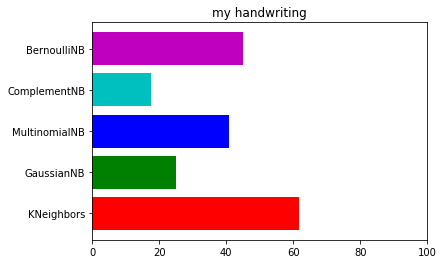
KNN이 가장 좋은 결과로 61.67%가 나왔다. 이런 류의 데이터셋에서는 확실히 KNN 이 강세긴 하지만..
역시 모든 알고리즘이 이미지를 예측하기에는 좋지 못한 결과를 나타냈다.
그냥 CNN을 사용하기로 하는게 좋은 선택이 될 것이다.....
그렇다면 이번에는 CNN을 이용해서 훈련시킨 다음 훈련 결과를 보자. 딥러닝을 이용하는 만큼 결과를 기대해보며 진행을 했다.
데이터 셋의 경우 저번과 같은 데이터를 이용해서 진행을 해 보았다. 전처리 과정은 지난글을 확인하길 바란다. 그럼 데이터를 불러와 보자.
import os
import cv2
import numpy as np
from sklearn.preprocessing import *

def createdataset(directory):       #sklearn사용을 위해 데이터세트를 생성
    files = os.listdir(directory)
    x = []
    y = []
    for file in files:
        attr_x = cv2.imread(directory+file, cv2.IMREAD_GRAYSCALE)
        ret , attr_x = cv2.threshold(attr_x,170,255,cv2.THRESH_BINARY) #영상 이진화
        attr_x = attr_x.reshape(32,32,1)
        attr_y = int(file[0])

        x.append(attr_x)
        y.append(attr_y)

    x = np.array(x)

    y = np.array([[i] for i in y])
    enc = OneHotEncoder(categories='auto')
    enc.fit(y)
    y = enc.transform(y).toarray()

    return x , y
train_dir = './kNN/trainingPNGs/'
train_x ,train_y = createdataset(train_dir)
test_dir = './kNN/testPNGs/'
test_x , test_y = createdataset(test_dir)
print('data set shape :',train_x.shape,train_y.shape,test_x.shape,test_y.shape)| data set shape : (1934, 32, 32, 1) (1934, 10) (120, 32, 32, 1) (120, 10) |
데이터를 모두 불러 온 후 tensorflow를 이용하여 CNN의 기본 모델인 3층짜리 모델을 구현해 보았다.
import tensorflow as tf
import random
import matplotlib.pyplot as plt

tf.set_random_seed(777) #reproducibility

X = tf.placeholder(tf.float32, [None, 32,32,1])
Y = tf.placeholder(tf.float32, [None, 10])
keep_prob = tf.placeholder(tf.float32)

#===============================================================================
W1 = tf.Variable(tf.random_normal([3, 3, 1, 16], stddev=0.01))
#표준편차가 0.01인 3x3매트릭스(깊이1) 데이터를 16개만큼 뽑겠다
#32x32x16
L1 = tf.nn.conv2d(X, W1, strides=[1, 1, 1, 1], padding='SAME')
#strides를 통해 축을 여러개 만들어 주어 이동방향을 여러방향으로 하게 했으나 가운데 1,1만 적용이 된다
#제로패딩을통해 사이즈를 동일하게 만듬
L1 = tf.nn.relu(L1)     #relu함수를 이용 음수값을 제거하는 방법으로 사용된다.
L1 = tf.nn.max_pool(L1, ksize=[1, 2, 2, 1], strides=[1, 2, 2, 1], padding='SAME')
#16x16x16
#컨벌루션된 결과를 max pooling을 통해 최댓값으로 다시 정리 1차원축으로 2칸 2차원축으로도 2칸이동한다
#제로패딩을 통해 크기가 줄지 않아야하지만 2x2필터를 사용하여서 크기가 반으로 줄어든다 depth는 그대로 유지된다(32)
#===============================================================================
W2 = tf.Variable(tf.random_normal([3, 3, 16, 32], stddev=0.01))
#역시 필터를 생성하는데 3x3매트릭스의 깊이가16인 데이터를 32개를 사용한다
#16x16x32
L2 = tf.nn.conv2d(L1, W2, strides=[1, 1, 1, 1], padding='SAME')
L2 = tf.nn.relu(L2)
L2 = tf.nn.max_pool(L2, ksize=[1, 2, 2, 1], strides=[1, 2, 2, 1], padding='SAME')
#8x8x32
#===============================================================================
#레이어 추가 부분
W3 = tf.Variable(tf.random_normal([3, 3, 32, 64], stddev =0.01))
L3 = tf.nn.conv2d(L2, W3, strides=[1, 1, 1, 1], padding='SAME') #7x7x64
L3 = tf.nn.relu(L3)
L3 = tf.nn.max_pool(L3, ksize = [1, 2, 2, 1], strides=[1, 2, 2, 1], padding='SAME')
#4x4x64
#===============================================================================
L3_flat = tf.reshape(L3,[-1, 4 * 4 * 64])

W4 = tf.Variable(tf.random_normal([4 * 4 * 64, 10],stddev=0.01))
# 최종 출력값 L2 에서의 출력 4*4*64개를 입력값으로 받아서 0~9 레이블인 10개의 출력값을 만듬
#===============================================================================
b = tf.Variable(tf.random_normal([10]))
hypothesis = tf.matmul(L3_flat, W4) +b
target1 = tf.argmax(tf.nn.softmax(hypothesis),1)

cost = tf.reduce_mean(tf.nn.softmax_cross_entropy_with_logits(logits = hypothesis,
                                                              labels = Y))
#costfunction
optimizer = tf.train.AdamOptimizer(learning_rate=learning_rate).minimize(cost)
#adamoptimizer를 사용 adam은 최적값의 근사치일때 넓게 점프해서 한번더 체크해준다
sess = tf.Session()
#세션을 통해 메모리에 설정한것들을 올려준다
sess.run(tf.global_variables_initializer())
tensorflow를 통해 모델 구현을 한 후 데이터를 집어넣어 훈련시켜 결과를 확인해보자!
learning_rate = 0.001   #러닝하면서 찾아갈 이동 단위
training_epochs = 20   #훈련을 시킬 횟수
batch_size = 64        #훈련시킬 데이터의 묶음

for epoch in range(training_epochs) :   #같은 트레이닝데이터를 epoch수만큼 훈련시킨다
    avg_cost = 0                        #오버피팅을 통한 정확도 상승을 목표로 한다
    total_batch = int(train_x.shape[0]/ batch_size)
    #train set에 example들을 batchsize(100)만큼 나누어주어 total batch를 구한다
    batch_start = 0
    batch_finish = batch_size

    for  i in range(total_batch) :      #전체 데이터를 100장씩 훈련시키게 된다
        batch_xs = train_x[batch_start:batch_finish]
        batch_ys = train_y[batch_start:batch_finish]
        feed_dict = {X:batch_xs, Y:batch_ys}    #placeholder로 설정한 그릇에 데이터 담아줌
        cost_val, _ ,hypo,tg = sess.run([cost,optimizer,hypothesis,target1],feed_dict=feed_dict)
        avg_cost += cost_val / total_batch      #출력을 위해 avg코스트를 만들어주어 확인

        batch_start += total_batch
        batch_finish += total_batch

        if batch_finish > train_x.shape[0] :
            batch_finish = -1

    print('Epoch :', '%04d'%(epoch+1),'cost = ','{:9f}'.format(avg_cost))


print('Learning Finished!!')        #5번의 훈련(epoch)을 모두 마치면 출력

correct_prediction = tf.equal(tf.argmax(hypothesis,1),tf.argmax(Y,1))
accuracy = tf.reduce_mean(tf.cast(correct_prediction,tf.float32))
print('Accuracy : ', sess.run(accuracy, feed_dict={X:test_x,
                                                   Y:test_y}))

r = random.randint(0,test_x.shape[0]-1)
print('Label : ',sess.run(tf.argmax(test_y[r:r+1],1)))
print('Prediction : ',sess.run(tf.argmax(hypothesis,1),
                               feed_dict={X:test_x[r:r+1]}))

plt.imshow(test_x[r:r+1].reshape(32,32),cmap = 'Greys',
           interpolation='nearest')
plt.show()| Epoch : 0001 cost = 1.234716 Epoch : 0002 cost = 0.148306 Epoch : 0003 cost = 0.068033 Epoch : 0004 cost = 0.045200 Epoch : 0005 cost = 0.035680 Epoch : 0006 cost = 0.017864 Epoch : 0007 cost = 0.009263 Epoch : 0008 cost = 0.009128 Epoch : 0009 cost = 0.004491 Epoch : 0010 cost = 0.012803 Epoch : 0011 cost = 0.013326 Epoch : 0012 cost = 0.019347 Epoch : 0013 cost = 0.015906 Epoch : 0014 cost = 0.016427 Epoch : 0015 cost = 0.015754 Epoch : 0016 cost = 0.039717 Epoch : 0017 cost = 0.009230 Epoch : 0018 cost = 0.005671 Epoch : 0019 cost = 0.000750 Epoch : 0020 cost = 0.000149 Learning Finished!! Accuracy : 0.675 Label : [1] Prediction : [1] |

간단하게 20epoch를 돌려 확인해 보았고 정확도는 67.5%로 출력 되었다. epoch를 늘려 보았지만 그 이상은 overfitting으로 인해 오히려 정확도가 낮아 졌다. 물론 20epoch의 결과도 사실 KNN의 정확도가 61.67%였기 때문에 별 차이가 없는 것을 확인할 수 있다.
이 것의 대한 이슈는 전적으로 데이터의 갯수 부족이라는 생각이 든다. 그렇다면 mnist의 데이터 전체를 훈련시켜 나의 손글씨를 인식 시켜 정확도를 확인해보자.
tensorflow에서 제공하는 mnist데이터의 갯수는 총 5만5000개로 이 데이터를 훈련시켜 확인해 보았다. 데이터의 갯수가 많이 늘었으므로 epoch또한 늘려 주었다.
from tensorflow.examples.tutorials.mnist import input_data

mnist = input_data.read_data_sets("MNIST_data/", one_hot = True)

for epoch in range(training_epochs) :
    avg_cost = 0
    total_batch = int(mnist.train._num_examples / batch_size)
    for  i in range(total_batch) :
        batch_xs, batch_ys = mnist.train.next_batch(batch_size)
        feed_dict = {X:batch_xs, Y:batch_ys}
        cost_val, _ ,hypo,tg = sess.run([cost,optimizer,hypothesis,target1],feed_dict=feed_dict)
        avg_cost += cost_val / total_batch

    print('Epoch :', '%04d'%(epoch+1),'cost = ','{:9f}'.format(avg_cost))

print('Learning Finished!!')

correct_prediction = tf.equal(tf.argmax(hypothesis,1),tf.argmax(Y,1))
accuracy = tf.reduce_mean(tf.cast(correct_prediction,tf.float32))
print('Accuracy : ', sess.run(accuracy, feed_dict={X:test_x,
                                                   Y:test_y}))

r = random.randint(0,test_x.shape[0]-1)
print('Label : ',sess.run(tf.argmax(test_y[r:r+1],1)))
print('Prediction : ',sess.run(tf.argmax(hypothesis,1),
                               feed_dict={X:test_x[r:r+1]}))

plt.imshow(test_x[r:r+1].reshape(28,28),cmap = 'Greys',
           interpolation='nearest')
plt.show()| Extracting MNIST_data/train-images-idx3-ubyte.gz Extracting MNIST_data/train-labels-idx1-ubyte.gz Extracting MNIST_data/t10k-images-idx3-ubyte.gz Extracting MNIST_data/t10k-labels-idx1-ubyte.gz Epoch : 0001 cost = 0.651246 Epoch : 0002 cost = 0.152724 Epoch : 0003 cost = 0.095623 Epoch : 0004 cost = 0.073589 Epoch : 0005 cost = 0.063206 Epoch : 0006 cost = 0.053531 Epoch : 0007 cost = 0.048459 Epoch : 0008 cost = 0.041821 Epoch : 0009 cost = 0.037713 Epoch : 0010 cost = 0.032538 ... Epoch : 0040 cost = 0.000237 Epoch : 0041 cost = 0.000042 Epoch : 0042 cost = 0.000011 Epoch : 0043 cost = 0.000008 Epoch : 0044 cost = 0.000006 Epoch : 0045 cost = 0.000005 Epoch : 0046 cost = 0.000004 Epoch : 0047 cost = 0.000003 Epoch : 0048 cost = 0.000003 Epoch : 0049 cost = 0.000002 Epoch : 0050 cost = 0.000002 Learning Finished!! Accuracy : 0.841 Label : [4] Prediction : [4] |

결과는 84.1%로 정확도가 꽤나 상승한 것을 알 수 있다. 하지만 역시 90% 이상이 아니기 때문에 만족스러운 결과는 아니었다. 이 경우의 문제는 1차적으로는 모델 자체가 CNN 3층 기본 모델로는 훈련이 잘 안될 가능성이 있다는 것, 그리고 테스트 데이터가 너무 부족하거나, 형태의 문제일 수 있다.
사실 mnist의 훈련데이터와 test데이터를 사용하면 99퍼센트는 10epoch만 돌려도 나온다. 여기까지 mnist를 이용하여 전처리와 머신러닝 딥러닝까지 해보았다. mnist를 통해 인공지능에 입문하는 사람이 많은 만큼 데이터를 이용하여 다양한 것을 해보는 것은 좋은 시도일 것이다.